Interpolation

Implementation: eko.interpolation

In order to obtain the operators in an PDF independent way we use approximation theory. Therefore, we define the basis grid

\[\mathbb G = \{ x_j : 0 < x_j <= 1, j=0,\ldots,N_{grid}-1 \}\]

from which we define our interpolation

\[f(x) \sim \bar f(x) \equiv \sum\limits_{j=0}^{N_{grid} - 1 } f(x_j) p_j(x)\]

Thus each grid point \(x_j\) has an associated interpolation polynomial \(p_j(x)\) (represented by eko.interpolation.BasisFunction). We interpolate in \(\ln(x)\) using Lagrange interpolation among the nearest \(N_{degree}+1\) points, which renders the \(p_j(x)\): polynomials of order \(O(\ln^{N_{degree}}(x))\).

Algorithm

First, we split the interpolation region into several areas (represented by eko.interpolation.Area), which are bound by the grid points:

\[A_j = (x_j,x_{j+1}], \quad \text{for}~j=0,\ldots,N_{grid}-2\]

Note, that we include the right border point into the definition, but not the left which keeps all areas disjoint. This assumption is based on the physical fact, that PDFs do have a fixed upper bound (\(x=1\)), but no fixed lower bound.

Second, we define the interpolation blocks, which will build the interpolation polynomials and contain the needed amount of points:

\[B_j = \{x_j,\ldots,x_{j+N_{degree}+1}\} \quad \text{for}~j=0,\ldots,N_{grid}-N_{degree}-2\]

Now, we construct the interpolation in a bottom-up approach for a given point \(\bar x\) for the interpolating function \(\bar f(\bar x)\). (The actual implementation is done in eko.interpolation.InterpolatorDispatcher)

1. Determine the relevant active area \(\bar A(\bar x)\) :

\[\bar A(\bar x) = A_j : \bar x \in A_j\]

2. Determine the associated block \(\bar B(\bar A)\) : Choose the block in which \(\bar A(\bar x)\) is located most central. For an odd number of \(N_{degree}\) choose the block which is located higher, i.e. closer to \(x=1\) (following the choice of borders for the areas). At the border of the grid, choose the “most central”.

3. Only the points and their associated polynomials which are in \(\bar B\) participate in the interpolation of \(\bar f(\bar x)\). All other polynomials vanish:

\[p_j(\bar x) = 0 \quad \text{for}~j : x_j \not\in \bar B\]

4. The active polynomials build a Lagrange interpolation over their associated points

\[p_j(\bar x) = \prod\limits_{j\neq k} \frac{\ln(\bar x) - \ln(x_k)}{\ln(x_j) - \ln(x_k)} \quad \text{for}~j,k : x_{j,k} \in \bar B\]

The generated polynomials are orthonormal in the following sense

\[p_j(x_k) = \delta_{jk}, \quad \text{for}~j,k=0,\ldots,N_{grid}-1\]

and thus continuous, however, they are not necessarily differentiable. They are also complete in the following sense

\[\sum\limits_{j=0}^{N_{grid}-1} p_j(x) = 1, \quad \text{for}~x \in (\text{min}(\mathbb G),\text{max}(\mathbb G)]\]

Example

To outline the interpolation algorithm, let’s consider the following example configuration:

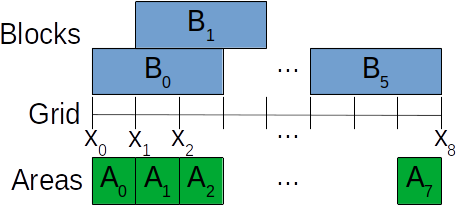
Example interpolation configuration with \(N_{grid}=9\) points using a polynomial of degree \(N_{degree}=3\) to interpolate. It has 8 areas and 6 blocks.

The mapping between areas and blocks are then given by

Mapping in the example configuration

A0 -> B0, A1 -> B0, A2 -> B1, A3 -> B2, A4 -> B3, A5-> B4, A6 -> B5, A7 -> B5

The generated polynomials then look like:

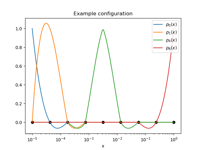
Selected polynomials of the example configuration. The 9 points have been placed logarithmically equidistant in \((10^{-5},1]\). Note that \(p_4(x)\) is still piecewise of degree 3.

Change Interpolation Basis

It is always possible to change interpolation basis, that corresponds to change interpolation grid.

The way it is done is the following:

\[\begin{split}f(x) \sim \bar f(x) &= \sum\limits_{j=0}^{N_{grid} - 1 } f(x_j) p_j(x)\\ \bar f(x) \sim \bar{\bar{f}}(x) &= \sum\limits_{k=0}^{\tilde{N}_{grid} - 1 } \bar f(\tilde{x}_k) \tilde{p}_k(x) = \sum\limits_{k=0}^{\tilde{N}_{grid} - 1 } \sum\limits_{j=0}^{N_{grid} - 1 } f(x_j) p_j(\tilde{x}_k) \tilde{p}_k(x)\end{split}\]

So the change of basis to apply to coefficients/polynomials is:

\[M_{jk} = p_j(\tilde{x}_k)\]

that corresponds to evaluate the old polynomials \(p_j\) (i.e. took the place of the continuous function in \(\bar f\)) on the new points \(\tilde x_k\).

Take care that in the above sections it has been explained that the target function is interpolated by approximating it with a piecewise polynomial.

Piecewise Polynomials Interpolation

It is very relevant to notice that it is not a polynomial, indeed being defined piecewise only the function is continuous, but not its derivatives.

Then even interpolating on a bigger but different grid might cause a further approximation.

Indeed no polynomial is able to produce a discontinuity in the derivatives, thus if an old grid point falls in the middle of a new grid area an approximation is expected (that intuitevely it would happen only if the grid were smaller, but it is also happening for larger poorly chosen ones).

Since further interpolating will cause a loss of accuracy it is recommended to have the new grid being a subset or a superset of the previous one, or in general to share as many points as possible.